 Buch kaufen
 Buch kaufen
 Buch kaufen
# invisible
import matplotlib as mpl
mpl.rcParams['figure.dpi'] = 300
Es war noch nie einfacher, ein Bild aufzunehmen als heute. Alles was Sie normalerweise brauchen ist ein Handy. Dies sind die Grundvoraussetzungen, um ein Bild aufzunehmen und anzusehen. Das Fotografieren ist kostenlos, wenn wir die Kosten für das Mobiltelefon nicht berücksichtigen, das ohnehin oft für andere Zwecke gekauft wird. Vor einer Generation brauchten Amateur- und echte Künstler spezielle und oft teure Ausrüstung, und die Kosten pro Bild waren alles andere als kostenlos.
Wir machen Fotos, um großartige Momente unseres Lebens in der Zeit zu konservieren. "Eingelegte Erinnerungen", die bereit sind, in Zukunft nach Belieben "geöffnet" zu werden.
Ähnlich wie beim Einmachen müssen wir die richtigen Konservierungsmittel verwenden. Natürlich bietet uns das Mobiltelefon auch eine Reihe von Bildverarbeitungssoftware, aber sobald wir eine große Anzahl von Fotos verarbeiten müssen, benötigen wir andere Tools. Hier kommen Programmierung und Python ins Spiel. Python und seine Module wie Numpy, Scipy, Matplotlib und andere Spezialmodule bieten die optimale Funktionalität, um mit der Flut von Bildern fertig zu werden.
Um Ihnen das notwendige Wissen zu vermitteln, befasst sich dieses Kapitel unseres Python-Tutorials mit der grundlegenden Bildverarbeitung und -manipulation. Zu diesem Zweck verwenden wir die Module NumPy, Matplotlib und SciPy.
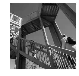
Wir beginnen mit dem scipy Paket misc. Die Hilfedatei besagt, dass scipy.misc verschiedene Dinge enthalte, die man sonstwo nicht unterbringen konnte. So enthält es auch beispielsweise ein paar Bilder, wie das folgende:
from scipy import misc
import matplotlib.pyplot as plt

ascent = misc.ascent()
plt.gray()
plt.imshow(ascent)
plt.show()
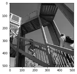
Zusätzlich zum Bild erkennen wir, dass die Ticks an den Achsen ebenfalls ausgegeben werden. Das ist sicherlich interessant, wenn Sie Informationen zur Größe und Pixel-Position benötigen, jedoch möchte man in den meisten Fällen das Bild ohne diese Informationen sehen. Indem wir den Befehl plt.axis("off") hinzufügen, können wir die Ticks und Achsen ausblenden:
from scipy import misc

ascent = misc.ascent()
import matplotlib.pyplot as plt
plt.axis("off") # removes the axis and the ticks
plt.gray()
plt.imshow(ascent)
plt.show()
Wir sehen, dass der Typ des Bildes ein Integer-Array ist:
ascent.dtype
Wir können auch die Größe des Bildes prüfen:
ascent.shape
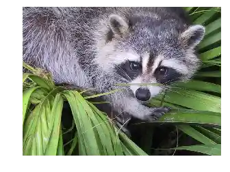
Das misc-Packet beinhaltet auch ein Bild eines Waschbären:
import scipy.misc
face = scipy.misc.face()
print(face.shape)
print(face.max)
print(face.dtype)
plt.axis("off")
plt.gray()
plt.imshow(face)
plt.show()
import matplotlib.pyplot as plt
import matplotlib.image as mpimg
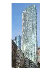
Matplotlib unterstützt nur PNG-Bilder.
img = mpimg.imread('frankfurt.png')
print(img[:3])
plt.axis("off")
imgplot = plt.imshow(img)
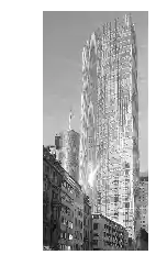
lum_img = img[:,:,1]
print(lum_img)
plt.axis("off")
imgplot = plt.imshow(lum_img)
Färbung, Schatten und Farbton
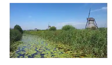
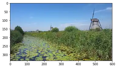
Jetzt möchten wir auf die Tönung eines Bildes eingehen. Tönung ist ein Ausdruck aus der Farb-Theorie ist eine oft von Malern verwendete Technik. Es ist kaum vorstellbar, wenn man an Maler denkt, gleichzeitig nicht an die Niederlande zu denken. Wir verwenden ein Bild mit "Holländischen Windmühlen" in unserem nächsten Beispiel. (Das Bild wurde in Kinderdijk aufgenommen, ein Dorf in den Niederlanden über 15km östlich von Rotterdam und über 50km entfernt von Den Haag. Es ist ein UNESCO Weltkulturerbe seit 1997.)
windmills = mpimg.imread('windmills.png')

plt.axis("off")
plt.imshow(windmills)
plt.imshow(windmills)
Wir möchten nun das Bild tönen. Das bedeutet wir "mischen" unsere Farben mit weiss. Dies wird die Helligkeit des Bildes erhöhen. Wir schreiben dafür eine Python-Funktion, welche ein Bild und eine Prozent-Angabe als Parameter entgegen nimmt. "percentage" auf 0 zu setzen, wird das Bild nicht verändern. Wenn Sie es auf eins setzen, wird das Bild vollständig aufgehellt:
import numpy as np
import matplotlib.pyplot as plt
import matplotlib.image as mpimg

def tint(imag, percent):
    """
    imag: the image which will be shaded
    percent: a value between 0 (image will remain unchanged
             and 1 (image will completely white)
    """
    tinted_imag = imag + (np.ones(imag.shape) - imag) * percent
    return tinted_imag

windmills = mpimg.imread('windmills.png')

tinted_windmills = tint(windmills, 0.8)
plt.axis("off")
plt.imshow(tinted_windmills)
plt.imshow(tinted_windmills)

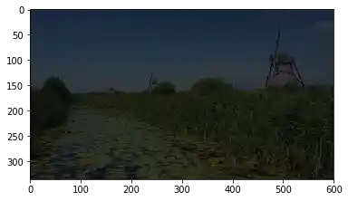
Ein Schatten ist eine Mischung einer Farbe mit Schwarz, was die Helligkeit verringert.
import numpy as np
import matplotlib.pyplot as plt
import matplotlib.image as mpimg

def shade(imag, percent):
    """
    imag: the image which will be shaded
    percent: a value between 0 (image will remain unchanged
             and 1 (image will be blackened)
    """
    tinted_imag = imag * (1 - percent)
    return tinted_imag

windmills = mpimg.imread('windmills.png')

tinted_windmills = shade(windmills, 0.7)
plt.imshow(tinted_windmills)
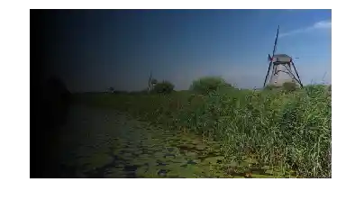
def vertical_gradient_line(image, reverse=False):
    """
    We create a horizontal gradient line with the shape (1, image.shape[1], 3))
    The values are incremented from 0 to 1, if reverse is False,
    otherwise the values are decremented from 1 to 0.
    """
    number_of_columns = image.shape[1]
    if reverse:
        C = np.linspace(1, 0, number_of_columns)
    else:
        C = np.linspace(0, 1, number_of_columns)
    C = np.dstack((C, C, C))
    return C

horizontal_brush = vertical_gradient_line(windmills)
tinted_windmills =  windmills * horizontal_brush
plt.axis("off")
plt.imshow(tinted_windmills)
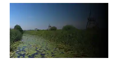
Wir werden das Bild von rechts nach links tönen indem wir den "reverse" Parameter der Python-Funktion auf "True" setzen:
def vertical_gradient_line(image, reverse=False):
    """
    We create a horizontal gradient line with the shape (1, image.shape[1], 3))
    The values are incremented from 0 to 1, if reverse is False,
    otherwise the values are decremented from 1 to 0.
    """
    number_of_columns = image.shape[1]
    if reverse:
        C = np.linspace(1, 0, number_of_columns)
    else:
        C = np.linspace(0, 1, number_of_columns)
    C = np.dstack((C, C, C))
    return C

horizontal_brush = vertical_gradient_line(windmills, reverse=True)
tinted_windmills =  windmills * horizontal_brush
plt.axis("off")
plt.imshow(tinted_windmills)
def horizontal_gradient_line(image, reverse=False):
    """
    We create a vertical gradient line with the shape (image.shape[0], 1, 3))
    The values are incremented from 0 to 1, if reverse is False,
    otherwise the values are decremented from 1 to 0.
    """
    number_of_rows, number_of_columns = image.shape[:2]
    C = np.linspace(1, 0, number_of_rows)
    C = C[np.newaxis,:]
    C = np.concatenate((C, C, C)).transpose()
    C = C[:, np.newaxis]
    return C

vertical_brush = horizontal_gradient_line(windmills)
tinted_windmills =  windmills
plt.imshow(tinted_windmills)
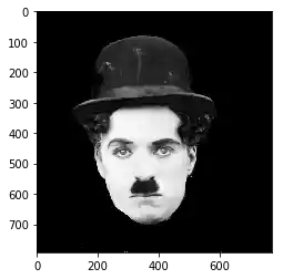
Ein Farbton wird entweder durch die Mischung einer Farbe mit Grau produziert, oder durch gleichzeitige Tönung und Schattierung.
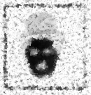
charlie = mpimg.imread('Chaplin.png')
plt.gray()
print(charlie)
plt.imshow(charlie)
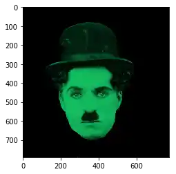
colored = np.dstack((charlie*0.1, charlie*1, charlie*0.5))

plt.imshow(colored)
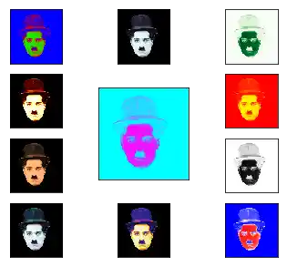
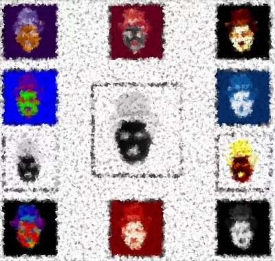
Im folgenden Beispiel werden verschiedene "colormaps" verwendet. Die "colormaps" befinden sich in matplotlib.pyplot.cm.datad:
plt.cm.datad.keys()
import numpy as np
import matplotlib.pyplot as plt

charlie = plt.imread('Chaplin.png')

#  colormaps plt.cm.datad
# cmaps = set(plt.cm.datad.keys())
cmaps = {'afmhot', 'autumn', 'bone', 'binary', 'bwr', 'brg',
         'CMRmap', 'cool', 'copper', 'cubehelix', 'Greens'}

X = [(4, 3, 1, (1, 0, 0)),
     (4, 3, 2, (0.5, 0.5, 0)),
     (4, 3, 3, (0, 1, 0)),
     (4, 3, 4, (0, 0.5, 0.5)),
     (4, 3, (5, 8), (0, 0, 1)),
     (4, 3, 6, (1, 1, 0)),
     (4, 3, 7, (0.5, 1, 0) ),
     (4, 3, 9, (0, 0.5, 0.5)),
     (4, 3, 10, (0, 0.5, 1)),
     (4, 3, 11, (0, 1, 1)),
     (4, 3, 12, (0.5, 1, 1))]

fig = plt.figure(figsize=(6, 5))

#fig.subplots_adjust(bottom=0, left=0, top = 0.975, right=1)
for nrows, ncols, plot_number, factor in X:
    sub = fig.add_subplot(nrows, ncols, plot_number)
    sub.set_xticks([])

    sub.imshow(charlie*0.0002, cmap=cmaps.pop())
    sub.set_yticks([])